Matching unpaired data with minimum entropy coupling
DDMEC (ICML 2025) solves minimum entropy coupling for continuous, high-dimensional data: given two unpaired datasets, it learns the joint distribution with the largest mutual information that is consistent with both. It is the most accurate method on PBMC multi-omics alignment, and it also translates images between unpaired domains.
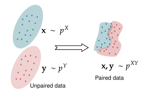
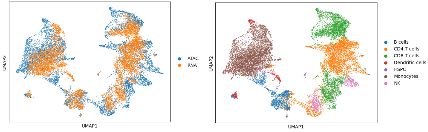
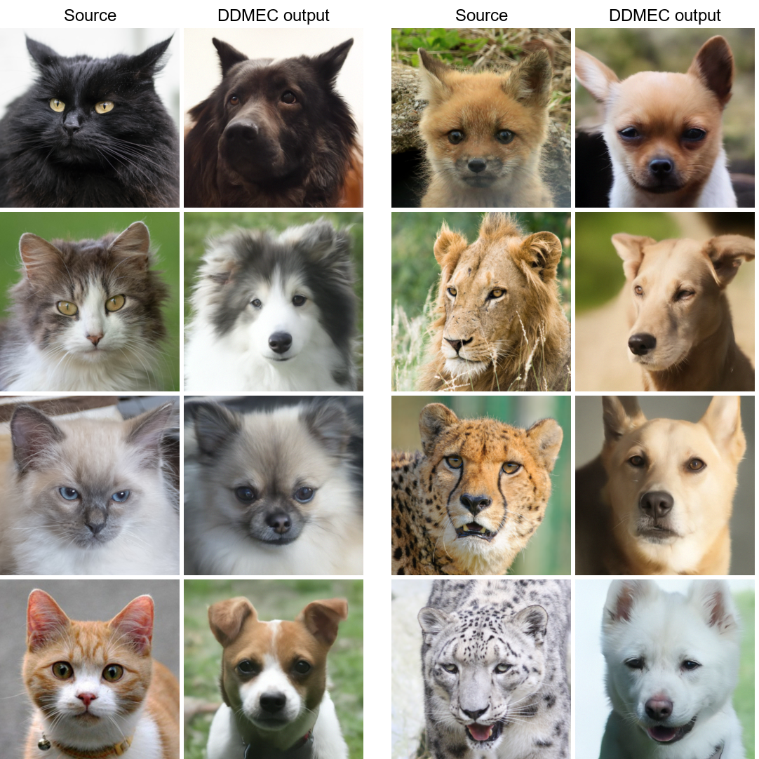
Single-cell experiments often measure gene expression (RNA) on one batch of cells and chromatin accessibility (ATAC) on another. Both describe the same biology, but no cell is measured twice, so there are no pairs to learn a mapping from. The same situation appears in unpaired image translation: we have many photos of cats and many photos of dogs, and no cat comes with its matching dog.
Minimum entropy coupling
Any joint distribution with marginals p_X and p_Y is a coupling of the two. There are infinitely many, from the independent product p_X \otimes p_Y to deterministic maps. Minimum entropy coupling picks the one with the smallest joint entropy:
\min_{p_{XY}} \ \mathbb H(p_{XY}) \quad \text{subject to} \quad \int p_{XY}(x,y)\,\mathrm dy = p_X(x), \ \ \int p_{XY}(x,y)\,\mathrm dx = p_Y(y).
Since I(X;Y) = \mathbb H(p_X) + \mathbb H(p_Y) - \mathbb H(p_{XY}) and the marginal entropies are fixed, this is the same as maximizing mutual information: pair the samples so that each one tells as much as possible about the other. It is a statistical criterion. Optimal transport answers a similar question geometrically, by minimizing a cost such as \mathbb E\lVert x - y\rVert^2, and therefore needs the two spaces to be comparable. Minimum entropy coupling needs no cost, and it works between spaces of different nature and dimension, such as RNA and ATAC profiles.
The problem is NP-hard for discrete variables, and almost all prior algorithms are for the discrete case. DDMEC addresses continuous, high-dimensional data. It avoids exactly deterministic couplings on purpose: a map y = g(x) satisfies the marginal constraints but gives a degenerate joint distribution.
Two models that train each other
We start by relaxing the marginal constraints into KL penalties, over a parametric family p^\theta_{XY}:
\min_\theta \ \mathbb H(p^\theta_{XY}) + \lambda_X \operatorname{KL}(p^\theta_X \,\|\, p_X) + \lambda_Y \operatorname{KL}(p^\theta_Y \,\|\, p_Y).
Writing p^\theta_{XY} = p^\theta_{X\mid Y}\, p_Y makes the Y marginal exact, and the joint entropy becomes a conditional entropy, which is the expected negative log-likelihood of a conditional generative model:
\min_\theta \ \mathbb E_{x,y \sim p^\theta_{XY}}\big[-\log p^\theta_{X\mid Y}(x \mid y)\big] + \lambda_X \operatorname{KL}(p^\theta_X \,\|\, p_X).
This factorization treats the two sides asymmetrically, so we add a second model in the opposite direction, p^\phi_{Y\mid X}\, p_X, and a penalty that keeps the two joints equal. When they agree, the gradient of the conditional entropy of one model can be computed with the likelihood of the other (Appendix A.1 of the paper). Each model is therefore trained to produce samples that the other model finds likely:
\min_\theta \ \mathbb E_{p^\theta_{XY}}\big[-\log p^\phi_{Y\mid X}\big] + \lambda_X \operatorname{KL}(p^\theta_X \,\|\, p^{\theta_*}_X), \qquad \min_\phi \ \mathbb E_{p^\phi_{XY}}\big[-\log p^\theta_{X\mid Y}\big] + \lambda_Y \operatorname{KL}(p^\phi_Y \,\|\, p^{\phi_*}_Y).
In practice this cooperative scheme is much more stable than training each model on its own entropy. The models p^{\theta_*}_X and p^{\phi_*}_Y are unconditional diffusion models pretrained on each dataset; they anchor the marginals and serve as the starting point for the conditional models.
Both conditionals are denoising diffusion models. The negative log-likelihood under the other model acts as a reward, so training amounts to reinforcement-learning fine-tuning of a diffusion model, with a policy gradient over the denoising steps. The likelihood is estimated from the denoising error, -\log p(x_0) \approx \text{const} + \tfrac12 \sum_t \mathbb E_\epsilon\lVert \epsilon - \epsilon_\theta(x_t, t)\rVert^2, and the marginal penalty is bounded by how far the fine-tuned noise predictions move from those of the pretrained model. A single training run gives the map in both directions.
Single-cell multi-omics
We test on PBMC (10x Multiome, RNA and ATAC, 11,910 cells) and on bone marrow CITE-seq (RNA and protein, 10,235 cells per modality). Each cell from one modality is mapped to the other, and we check whether its nearest neighbors there have the same cell-type label.
| Method | PBMC cell type | PBMC subtype | BM cell type | BM subtype |
|---|---|---|---|---|
| UnionCom | 34.8 ± 10.9 | 22.9 ± 7.2 | 51.8 ± 3.7 | 20.9 ± 2.6 |
| MMD-MA | 28.3 ± 6.4 | 10.2 ± 4.8 | 38.8 ± 17.9 | 10.4 ± 8.4 |
| SCOT | 12.9 ± 1.1 | 2.4 ± 0.2 | 90.5 ± 0.0 | 31.6 ± 0.0 |
| scTopoGAN | 61.7 ± 8.6 | 41.3 ± 6.5 | 50.9 ± 14.7 | 22.5 ± 5.4 |
| DDMEC | 66.3 ± 2.6 | 46.0 ± 0.5 | 77.3 ± 0.1 | 44.2 ± 0.1 |
DDMEC is the most accurate in three of the four columns; SCOT is better on bone marrow cell types. On SNARE-seq, where the true pairing is known, DDMEC has the lowest alignment error (FOSCTTM 0.147).
Unpaired image translation
On AFHQ and CelebA-HQ at 256 \times 256 we follow the evaluation protocol of EGSDE.
| Task | Best baselines (FID / SSIM) | DDMEC (FID / SSIM) |
|---|---|---|
| Cat → dog | SDDM 62.29 / 0.422; StarGAN v2 54.88 / 0.27 | 57.89 / 0.397 |
| Wild → dog | SDDM 57.38 / 0.328 | 59.22 / 0.346; 62.03 / 0.360 |
| Male → female | EGSDE 41.93 / 0.574 | 34.86 / 0.549; 40.73 / 0.593 |
Among diffusion-based methods DDMEC has the best FID on cat to dog and on male to female. On cat to dog the GAN baseline StarGAN v2 reaches a lower FID, with a much lower SSIM.
References
- M. Bounoua, G. Franzese, P. Michiardi. Learning to Match Unpaired Data with Minimum Entropy Coupling. ICML 2025. arXiv:2503.08501, code.
- A. Singh et al. scTopoGAN: unsupervised manifold alignment of single-cell data. 2023.
- Y. Choi, Y. Uh, J. Yoo, J.-W. Ha. StarGAN v2: Diverse Image Synthesis for Multiple Domains (AFHQ dataset). CVPR 2020.