Estimating information with diffusion processes

Over the past few years our group has written a series of papers on estimating information-theoretic quantities with diffusion models: mutual information first, then O-information, transfer entropy, discrete data, function spaces, and most recently an estimator that needs no training at all. The quantities look different, but every one of these methods rests on the same identity. This page derives it once. The pages linked at the bottom take one quantity each.

Everything is a KL divergence

For two probability measures \mu \ll \rho,

\operatorname{KL}(\mu \,\|\, \rho) = \mathbb{E}_{\mu}\!\left[\log \frac{\mathrm{d}\mu}{\mathrm{d}\rho}\right].

Mutual information is \operatorname{KL}(\mu^{XY} \,\|\, \mu^X \otimes \mu^Y). Differential entropy is a KL divergence to a Gaussian reference, plus a known constant. Total correlation, transfer entropy, and the terms of information decompositions are sums or conditional averages of KL divergences. A good estimator of KL divergence from samples gives all of them.

The obvious routes do not work well in high dimension. Estimating both densities and plugging them in needs a sample size that grows exponentially with the dimension. Variational bounds such as Donsker-Varadhan, \operatorname{KL}(\mu\|\rho) = \sup_T \mathbb{E}_\mu[T] - \log \mathbb{E}_\rho[e^T], replace the density ratio with a learned critic, but the Monte Carlo estimate of \log \mathbb{E}_\rho[e^T] has high variance. There is also a hard limit: a high-confidence lower bound above \log N nats cannot be certified from N samples (McAllester and Stratos, 2020).

The identity

We noise both distributions with the same Ornstein-Uhlenbeck process,

\mathrm{d}X_t = -X_t\,\mathrm{d}t + \sqrt{2}\,\mathrm{d}W_t, \qquad X_0 \sim \mu \ \text{or}\ \rho,

and look at the two path measures \mathbb{P}^\mu and \mathbb{P}^\rho on [0,T]. The argument takes three steps.

The two processes have the same transition kernel and differ only in where they start. The density ratio of two paths therefore reduces to the ratio of their initial points, and \operatorname{KL}(\mathbb{P}^\mu \| \mathbb{P}^\rho) = \operatorname{KL}(\mu \| \rho).

The KL divergence between path measures does not change if we reverse time. The reversed process is again a diffusion, and its drift contains the score of the noised marginal:

\mathrm{d}\hat X_t = \big(\hat X_t + 2\,\nabla \log p_{T-t}(\hat X_t)\big)\,\mathrm{d}t + \sqrt{2}\,\mathrm{d}\hat W_t .

The two reversed processes share the same noise and differ only in their drifts, by 2(\nabla\log p_t - \nabla \log q_t). Girsanov’s theorem gives the KL divergence between them as the expected integrated squared drift difference, divided by twice the squared diffusion coefficient. Putting the pieces together,

\operatorname{KL}(\mu \,\|\, \rho) = \int_0^T \mathbb{E}_{p_t}\!\big[\,\lVert \nabla \log p_t(X_t) - \nabla \log q_t(X_t) \rVert^2\,\big]\,\mathrm{d}t \;+\; \operatorname{KL}(p_T \,\|\, q_T).

Both noised laws converge exponentially fast to a standard Gaussian, so the last term vanishes as T grows. The same formula can also be obtained without path measures: differentiate \operatorname{KL}(p_t\|q_t) in time using the Fokker-Planck equation, integrate by parts, and integrate back from 0 to \infty.

A numerical check on two Gaussians, where the KL divergence is known in closed form:

Left: p_0 = \mathcal N(1.5, 0.5^2) is noised toward q_0 = \mathcal N(0,1), which is the stationary law. Right: the integrand \mathbb E_{p_t}\lVert s^p_t - s^q_t\rVert^2 over diffusion time. The area under the curve is 1.443 nats, equal to the closed-form value.

Turning it into an estimator

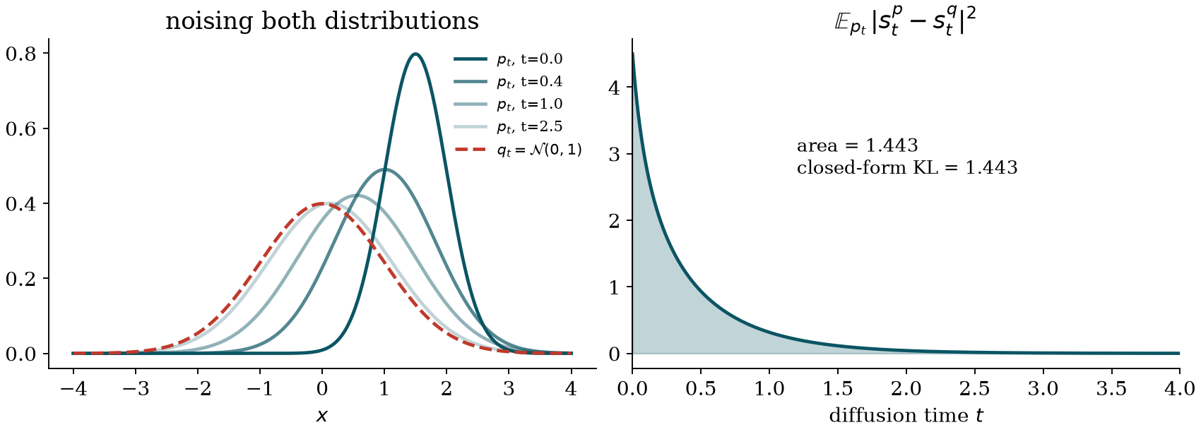
The scores are unknown, but learning them is exactly what a diffusion model does. By Tweedie’s formula the score of the noised law is an affine function of the optimal denoiser,

\nabla \log p_t(x) = \frac{e^{-t}\,\mathbb{E}[X_0 \mid X_t = x] - x}{1 - e^{-2t}},

so a network trained with the usual denoising loss \mathbb{E}\lVert \mathrm{net}_\theta(X_t, t) - X_0 \rVert^2 provides the scores we need. The estimate is then a Monte Carlo average of T \lVert s^p_t - s^q_t \rVert^2 over data points, diffusion times t \sim \mathcal U[0,T], and noise draws.

In practice two details make a difference. The integrand is largest at small t, where the learned scores are least accurate, so we sample t with importance weights. And we rarely train separate networks: with a conditioning flag, as in classifier-free guidance, one model returns the joint, marginal, and conditional scores that a given quantity requires.

The estimators

Each method applies the identity to a different pair of distributions.

Quantity	Compared distributions	Method	Venue
Mutual information, entropy	joint vs product of marginals; data vs Gaussian	MINDE	ICLR 2024
O-information	joint vs product of marginals, and joint vs product of full conditionals	SΩI	ICML 2024, oral
Transfer entropy	future given both pasts vs future given its own past	TENDE	AISTATS 2026
Integrated information decomposition	nine mutual informations between present and future	DIPHINE	preprint, 2026
Discrete data	as above, with a continuous-time Markov chain	INFO-SEDD	ICLR 2026
Coupling unpaired data	mutual information maximized under fixed marginals	DDMEC	ICML 2025
Trajectories	two laws on a function space	Functional KL	ICML 2026
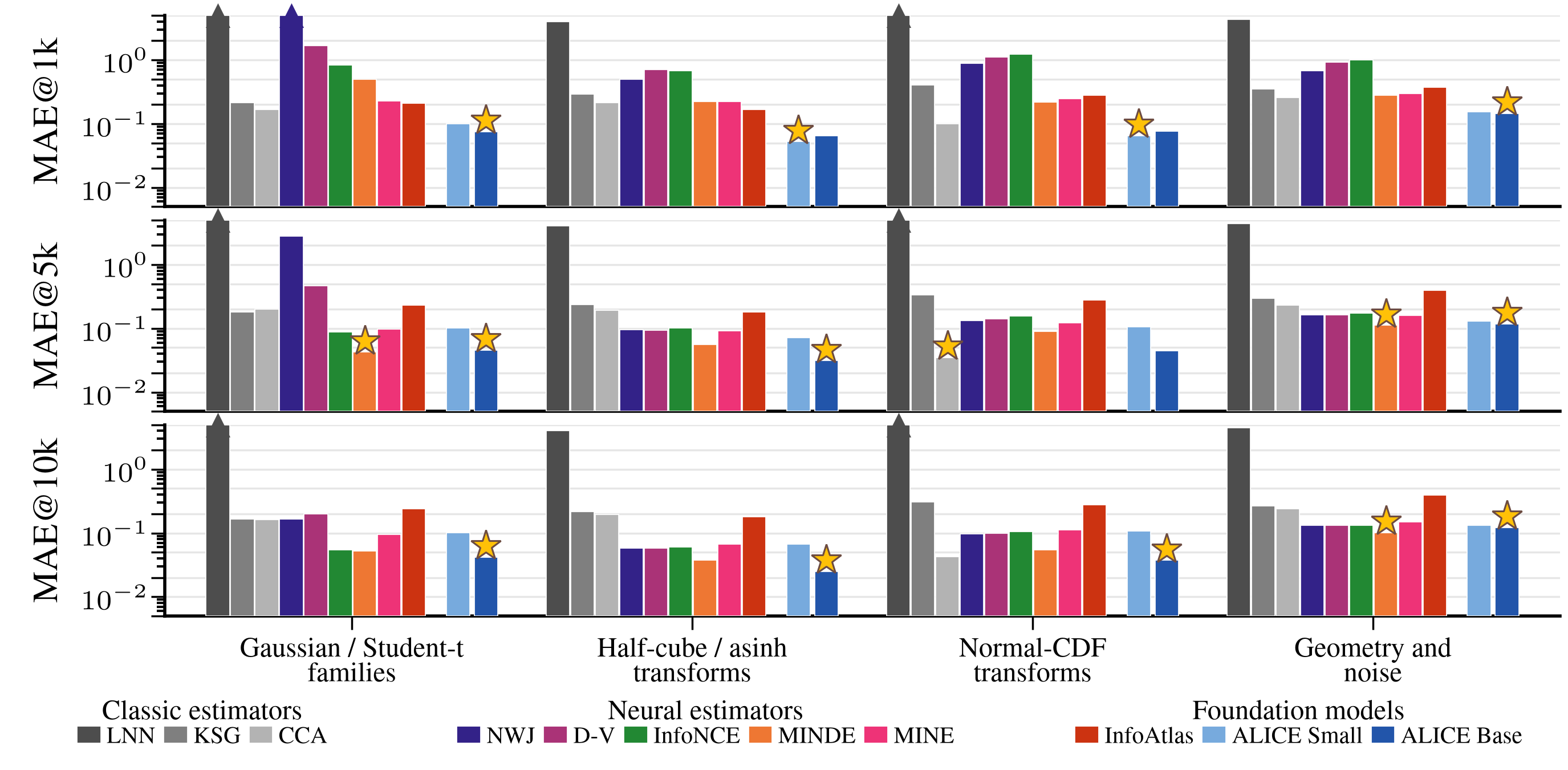
Mutual information, no training	the identity in velocity form, learned once for all distributions	ALICE	preprint, 2026

If you arrived here with a concrete question, this is roughly where to start:

Question	Start with
How much does Y tell me about X?	MINDE, or ALICE if you have few samples or do not want to train
Is the information in this system shared or only available jointly?	SΩI
Does the past of one signal help predict another?	TENDE
How do two coupled processes store, exchange, and integrate information?	DIPHINE
My data are sequences of symbols (DNA, text, spins)	INFO-SEDD
I have two datasets of the same objects but no pairs	DDMEC
Two models produce the same snapshots; do they produce the same dynamics?	Functional KL