Relative entropy between laws of trajectories

Snapshot data do not tell how cells move. Functional KL estimates the KL divergence between distributions of whole trajectories, and shows that methods with the same snapshot scores can have very different dynamics.

Functional KL (ICML 2026) estimates the KL divergence between two probability distributions over whole trajectories, using only the velocity fields of two functional flow-matching models. We use it to evaluate trajectory inference, where the usual snapshot metrics cannot tell correct dynamics from wrong ones.

Paper · Code

Single-cell RNA sequencing destroys the cell it measures. A time-course experiment therefore gives snapshots: cells sampled at a few time points, each observed once. Trajectory inference tries to reconstruct how the population moved between snapshots. Infinitely many distributions over trajectories agree with any finite set of snapshots, so the data alone do not identify the dynamics.

A snapshot: at each time, a cloud of states, and each sample is a single point x(t).

In function space each sample is a whole trajectory, and a model is a probability distribution over trajectories.

Why snapshot metrics are not enough

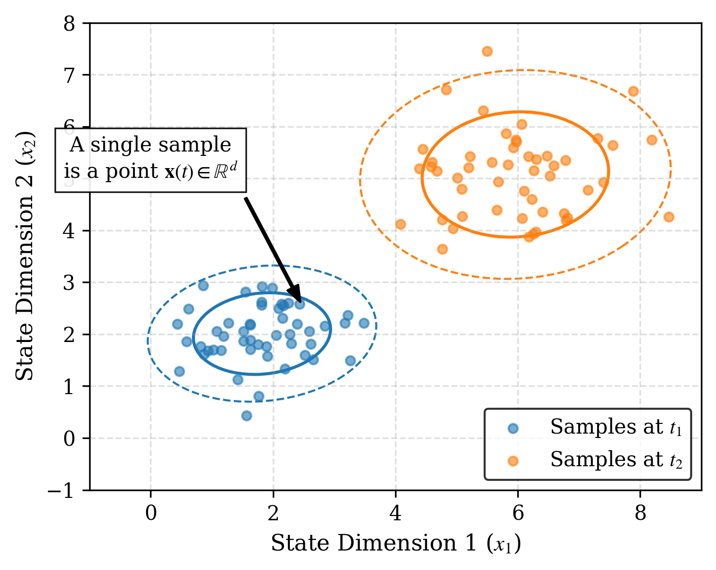
Methods are usually compared on held-out time points, with Wasserstein distances or MMD between predicted and observed snapshots. These scores ignore how the states at different times are connected. Two methods can put their samples in the same places at every time and still move them along very different paths.

The Petal benchmark at \tau = 0.75: ground-truth paths (black), MSBM (blue), and TIGON (red). Both methods match the snapshot almost equally well (W_2 0.160 and 0.155), but TIGON moves along smooth straight lines while the true paths are noisy. The reverse KL between the trajectory distributions tells them apart: 17.1 for MSBM, 35.5 for TIGON.

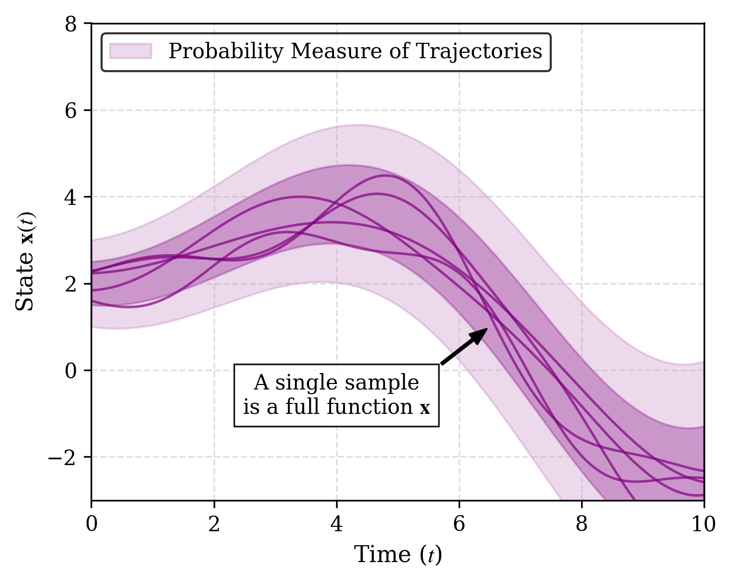
What we want instead is the KL divergence between the distribution of inferred trajectories \nu^B and a reference distribution \nu^A. Trajectories live in an infinite-dimensional space, where there is no Lebesgue measure and hence no density, so the KL divergence has to be written through the Radon-Nikodym derivative, \operatorname{KL}(\nu^A\|\nu^B) = \int_H \log \frac{\mathrm d\nu^A}{\mathrm d\nu^B}\,\mathrm d\nu^A. Even absolute continuity is delicate there: two Gaussian measures on a function space are typically mutually singular.

The estimator

The construction builds on generative diffusion models defined directly on function spaces, which we introduced with continuous-time functional diffusion processes (NeurIPS 2023) and reviewed in a survey on diffusion models in infinite dimensions (Philosophical Transactions A, 2025).

Let H be a separable Hilbert space and X_0 \sim \mu_0 = \mathcal N(0, C) a Gaussian with trace-class covariance C, whose Cameron-Martin space we write H_{\mu_0}. Functional flow matching moves noise to data along X_t = (1-t)X_0 + t X_1, with velocity v_t(x) = (\mathbb E[X_1 \mid X_t = x] - x)/(1-t). We train one such velocity field for X_1 \sim \nu^A and one for X_1 \sim \nu^B, starting from the same noise. Then

\operatorname{KL}(\nu^A \,\|\, \nu^B) = \int_0^1 \int_H \frac{t}{1-t}\, \big\lVert v^A_t(x) - v^B_t(x) \big\rVert^2_{H_{\mu_0}}\, \mathrm d\mu^A_t(x)\,\mathrm dt .

This holds when \nu^A \ll \nu^B and both distributions are concentrated on the Cameron-Martin space of the noise; in practice we choose a noise that is rougher than the data but still trace-class. The proof has three parts: the noised distributions stay mutually absolutely continuous at every t; the time derivative of the KL divergence can be written through the continuity equation; and the difference of log-density gradients with respect to the Gaussian reference equals \frac{t}{1-t}\,C^{-1}(v^A_t - v^B_t). It is the function-space version of the identity behind MINDE.

On the practical side, one neural operator represents both fields, with a binary flag choosing A or B. We use a mesh-informed neural operator, which handles irregular grids. The weight t/(1-t) diverges at t = 1; imposing v(x,1) = x through the parameterization v(x,t) = x + m(x,t) - m(x,1) removes the problem. The estimate is a Monte Carlo average over trajectories, times, and noise draws, with norms computed in a truncated Fourier basis, and it never simulates a path.

Does it recover known values?

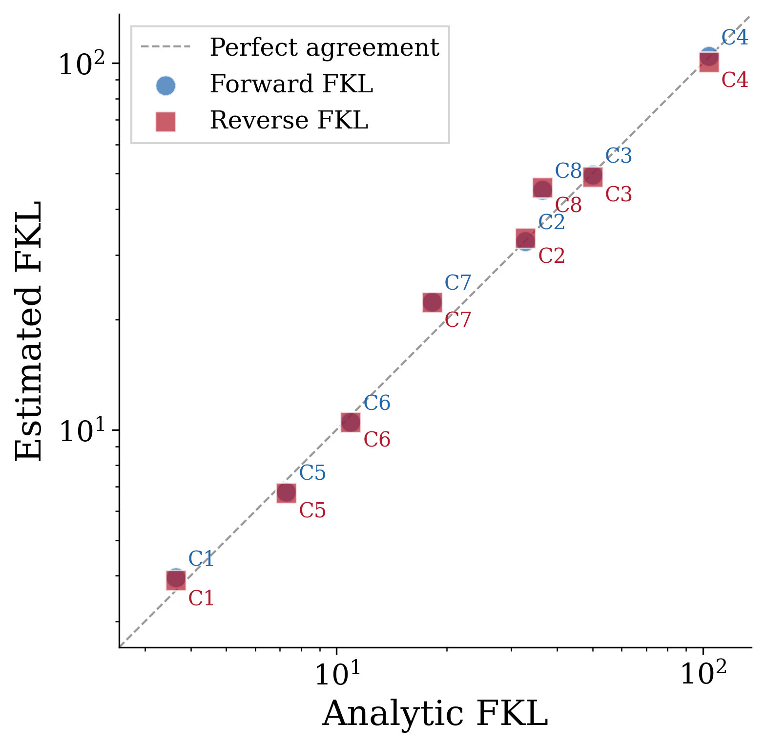
For Gaussian measures on function space the KL divergence has a closed form, so we can check the estimator directly.

Estimated against closed-form KL for eight Gaussian cases, forward (circles) and reverse (squares). The dashed line is perfect agreement.

KL between Gaussian measures on function space, selected cases from Table 1 of the paper.

Case	Dimension	Closed form	Forward	Reverse
1	1	3.64	3.95	3.88
2	1	32.79	32.61	33.31
3	1	50.00	49.58	49.00
4	1	103.74	104.46	100.58
6	3	10.93	10.48	10.49
8	10	36.43	45.12	45.73

The agreement is close in one dimension, and the estimator overestimates as the dimension grows (45.1 against 36.4 at dimension 10).

The second test uses linear SDEs, \mathrm dY_t = c\,Y_t\,\mathrm dt + g\,\mathrm dW_t, where the KL divergence between the path laws of two drifts c_A and c_B is also known. Here the two directions differ a lot, since one process is much more spread out than the other.

Estimated against closed-form KL for five linear SDE cases, forward (circles) and reverse (squares).

KL between path laws of linear SDEs, from Table 1 of the paper.

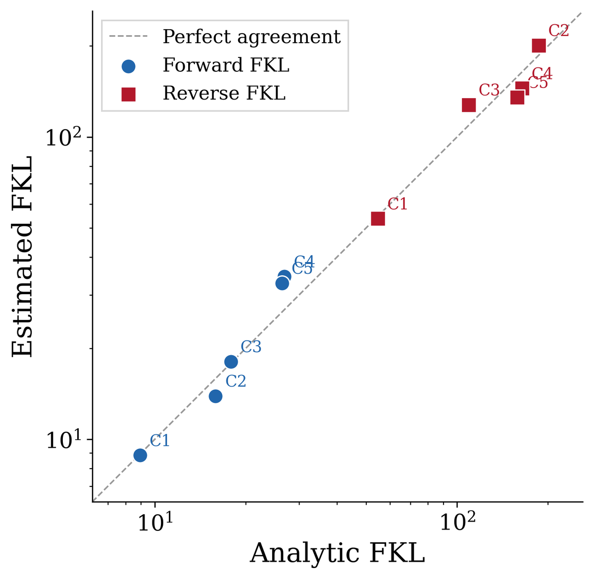
Case	Dimension	Forward, closed form	Forward, estimate	Reverse, closed form	Reverse, estimate
1	1	8.93	8.87	54.71	53.77
2	1	15.89	13.89	186.19	200.64
3	2	17.86	18.05	109.43	127.67
4	3	26.79	34.58	164.14	145.06
5	5	26.34	32.82	158.22	135.28

The first case is almost exact; in the others the error is roughly 7 to 20%.

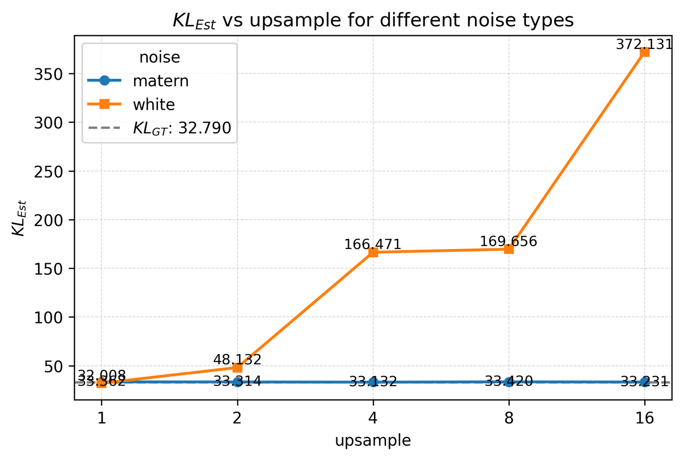
The noise has to be trace-class. The theory requires the noise covariance to be trace-class, and the experiments show what happens otherwise. We train on one grid and evaluate the same Gaussian case on grids up to sixteen times finer. With a rough Matérn noise the estimate stays between 33.1 and 33.4 against a true value of 32.79, at every resolution. With white noise it grows from 32.0 to 372.

Estimated KL as the evaluation grid is refined, for Matérn and white noise. The dashed line is the true value, 32.79.

Evaluating trajectory inference

We use Functional KL to compare six trajectory inference methods (vSB, SBIRR, MSBM, MFL, Action Matching, TIGON) against a reference. On the synthetic systems the reference is the true process, and VAL denotes fresh samples from it, which should receive the smallest divergence.

Forward / reverse Functional KL on the synthetic benchmarks (Table 2 of the paper); bold marks the best method other than VAL.

Method	Lotka-Volterra	Repressilator	Petal
VAL	0.27 / 0.27	0.02 / 0.01	0.08 / 0.08
SBIRR	43.4 / 42.8	23.5 / 25.2	16.0 / 49.4
vSB	165.1 / 126.9	82.9 / 79.0	18.9 / 53.4
MSBM	79.9 / 46.0	90.0 / 49.4	9.6 / 17.1
MFL	43.9 / 130.6	63.1 / 84.6	42.7 / 68.2
AM	44.9 / 55.5	66.9 / 126.2	12.3 / 31.6
TIGON	179.4 / 65.4	54.5 / 42.8	96.1 / 35.5

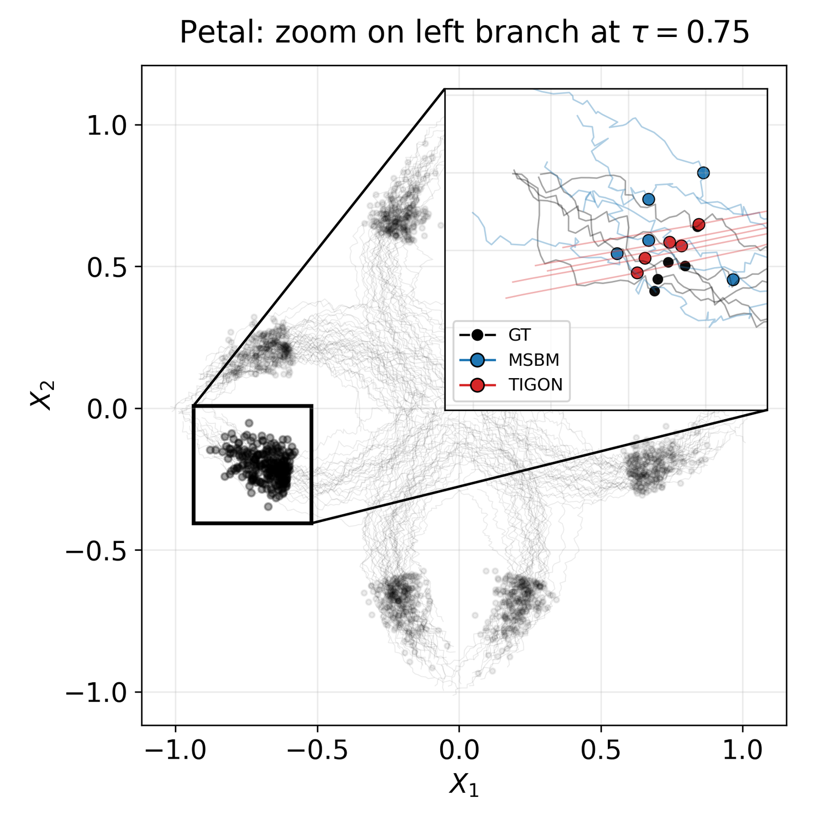
VAL receives the smallest divergence on every system. Among the methods, SBIRR is best on Lotka-Volterra and on the repressilator, and MSBM on Petal. Snapshot metrics give a different picture. On the repressilator, they rank TIGON above SBIRR, but TIGON produces a smooth spiral, while the true system oscillates between the three genes. The two are easy to tell apart when the trajectories are plotted.

Repressilator trajectories: ground truth, fresh samples (VAL), and the six methods, colored by time. TIGON (right) produces a smooth spiral, while the true system oscillates between the three genes.

On real single-cell data (embryoid body, hESC, mouse erythroid, human fibroblast) there is no ground truth, and the reference is a set of SBIRR trajectories.

Inferred trajectories on hESC data in the first three principal components, colored by time, with the observed snapshots as dots.

Forward / reverse Functional KL on real single-cell data, with SBIRR trajectories as reference (Table 3 of the paper).

Method	Embryoid body	hESC	Mouse erythroid	Human fibroblast
vSB	23.8 / 27.7	127.2 / 124.1	51.1 / 48.1	57.0 / 41.6
MSBM	29.5 / 21.5	111.2 / 81.7	65.6 / 37.6	58.9 / 26.8
MFL	22.1 / 73.2	97.1 / 117.9	42.3 / 79.3	29.7 / 69.8
AM	74.8 / 32.2	145.6 / 283.3	89.2 / 81.8	73.2 / 66.9
TIGON	122.5 / 41.1	293.1 / 161.7	250.6 / 82.4	197.8 / 69.5

On hESC, TIGON is the best method under every snapshot metric at one validation time, and the worst under Functional KL, because it produces smooth paths where the reference is noisy. More generally, rankings based on snapshot metrics change with the validation time, the metric, and its hyperparameters, while the Functional KL rankings agree with what one sees in the plots.

The two directions of the divergence answer different questions. The forward KL penalizes missing parts of the reference, and ranks MFL first on all four datasets. The reverse KL penalizes trajectories that wander outside the reference, and ranks MSBM first on all four.

Beyond trajectory inference, the same estimator applies to any pair of distributions over curves or fields, as long as both are concentrated on the Cameron-Martin space of a trace-class noise.

References

• C. Wang, L. Nepote, G. Franzese, P. Michiardi. Relative Entropy Estimation in Function Space: Theory and Applications to Trajectory Inference. ICML 2026. arXiv:2604.20775, code.
• G. Kerrigan, G. Migliorini, P. Smyth. Functional Flow Matching. 2023.
• G. Franzese, G. Corallo, S. Rossi, M. Heinonen, M. Filippone, P. Michiardi. Continuous-Time Functional Diffusion Processes. NeurIPS 2023. arXiv:2303.00800, code.
• G. Franzese, P. Michiardi. Generative diffusion models in infinite dimensions: a survey. Philosophical Transactions of the Royal Society A, 383(2299), 2025. doi:10.1098/rsta.2024.0322.