Redundancy and synergy: estimating O-information
SΩI (ICML 2024, oral) estimates O-information, the balance between redundancy and synergy in a system of many variables, with a single diffusion model. It works with high-dimensional variables, where estimators built from pairwise mutual informations break down.
Take three neurons. If all three carry the same signal, observing any one of them tells you everything, and the information is redundant. If instead the signal is the XOR of two of them, each neuron alone tells you nothing and every pair of variables looks independent: the information is synergistic, and it only appears when you look at the variables jointly. Pairwise measures miss this completely. O-information is a single number that captures the balance between the two, for any number of variables.
Definition
Let X = \{X^1, \dots, X^N\}, where each X^i can itself be a vector, and write X^{\setminus i} for all variables except X^i. Two classical extensions of mutual information to many variables are the total correlation
\mathcal T(X) = \sum_{i=1}^N \mathcal H(X^i) - \mathcal H(X) = \operatorname{KL}\Big(p(x) \,\Big\|\, \prod_{i=1}^N p(x^i)\Big)
and the dual total correlation
\mathcal D(X) = \mathcal H(X) - \sum_{i=1}^N \mathcal H\big(X^i \mid X^{\setminus i}\big).
Rosas et al. (2019) defined the O-information as their difference, \Omega(X) = \mathcal T(X) - \mathcal D(X). When \Omega > 0 the system is dominated by redundancy, and when \Omega < 0 by synergy. For three variables it coincides with the interaction information.
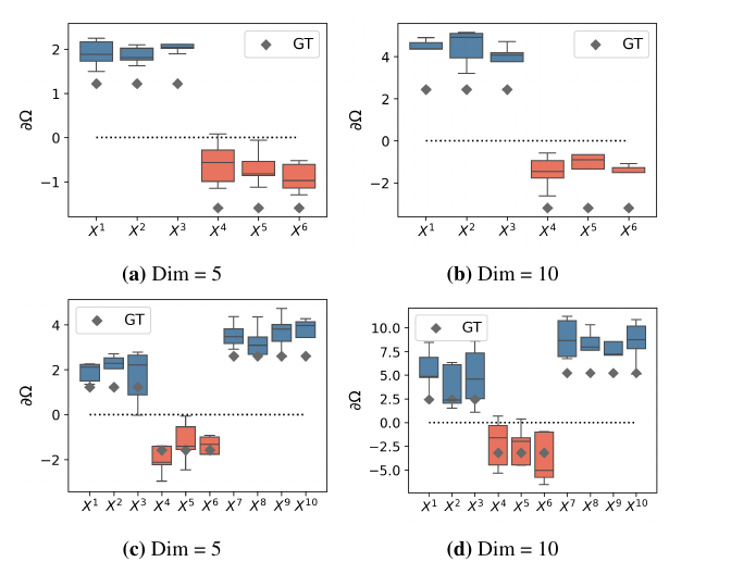
Partial information decomposition gives a finer picture, but it requires splitting the variables into sources and a target, and the number of terms grows rapidly: there are more than 10^{31} for nine variables. O-information needs no such split and stays a single number as N grows. Its gradient, \partial_i \Omega(X) = \Omega(X) - \Omega(X^{\setminus i}) (Scagliarini et al., 2023), tells which variables contribute redundancy (positive values) and which take part in synergistic interactions (negative values).
Until recently, O-information could only be computed for discrete data, by binning, or under a Gaussian assumption. The alternative of writing it as a sum of 2(N-1) mutual informations, each estimated by a separate neural network, accumulates the biases of all of them and inherits the limits of bound-based estimators in high dimension.
The estimator
Both terms are KL divergences between the joint distribution and a reference built from simpler pieces: the product of the marginals for \mathcal T, and the product of the full conditionals for \mathcal D. With the identity behind this series, each becomes an integrated squared difference of scores. Writing \tilde x for the sample noised at diffusion time t, and [\cdot^i]_{i=1}^N for the concatenation of per-variable blocks,
\mathcal T(X) = \int_0^T \frac{g_t^2}{2}\, \mathbb E\Big\lVert \nabla \log p_t(\tilde x) - \big[\nabla_{\tilde x^i} \log p_t(\tilde x^i)\big]_{i=1}^N \Big\rVert^2 \mathrm dt,
\mathcal D(X) = \int_0^T \frac{g_t^2}{2}\, \mathbb E\Big\lVert \nabla \log p_t(\tilde x) - \big[\nabla_{\tilde x^i} \log p_t(\tilde x^i \mid x^{\setminus i})\big]_{i=1}^N \Big\rVert^2 \mathrm dt ,
where in \mathcal D each block is noised while the others stay clean, and g_t is the diffusion coefficient of the noising process. O-information is the difference of the two.
This requires 2N+1 scores: the joint one, N marginals, and N full conditionals. We train a single network for all of them. Every variable gets its own diffusion time, and the vector of times \tau \in \mathbb R^N decides which score the network returns:
| Score | Diffusion times \tau | Other variables |
|---|---|---|
| Joint | [t, \dots, t] | noised together |
| Conditional of X^i | t for X^i, 0 for the rest | clean |
| Marginal of X^i | t for X^i, T for the rest | pure noise |
During training we pick one of these configurations at random at every step. The gradient of O-information needs a few more conditional scores, which we add to the same training.
Synthetic benchmarks
We test on Gaussian systems where O-information has a closed form: a redundant system (several variables are noisy copies of a shared source), a synergistic one (one variable is the sum of the others plus independent sources), and a mixed one, where synergy is fixed and redundancy grows until \Omega changes sign. The baselines write O-information as 2(N-1) mutual informations and estimate each with MINE, NWJ, InfoNCE, or CLUB.
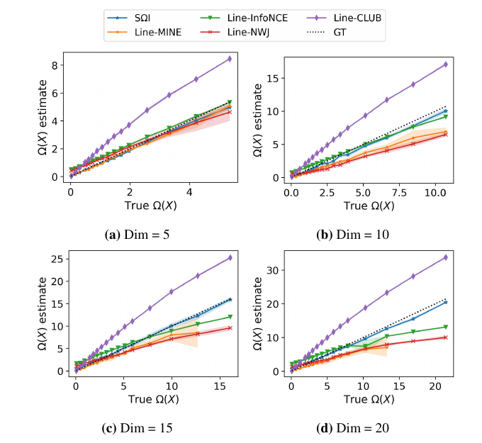
On the synergistic system several baselines get even the sign wrong in high dimension. On the mixed system SΩI follows the change of sign. The estimates remain good after nonlinear invertible transformations of the data (half-cube and normal CDF), with some bias for strongly synergistic systems under the half-cube map. About 10k training samples give a good trade-off between bias and variance.
Visual cortex
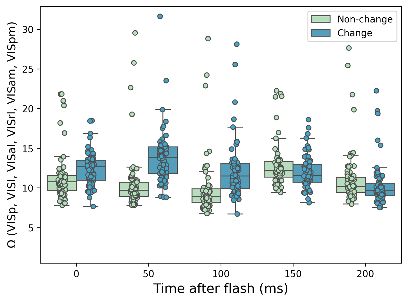
The main application in the paper is in neuroscience. In the Allen Institute Visual Behavior Neuropixels recordings, mice watch natural images that flash for 250 ms every 750 ms, and are rewarded for reporting when the image changes. We average spike counts over the units of each visual area in 2 ms steps, so that each area becomes a 25-dimensional variable in each 50 ms window after a flash, and estimate the O-information of three areas (VISp, VISl, VISal) and of all six.
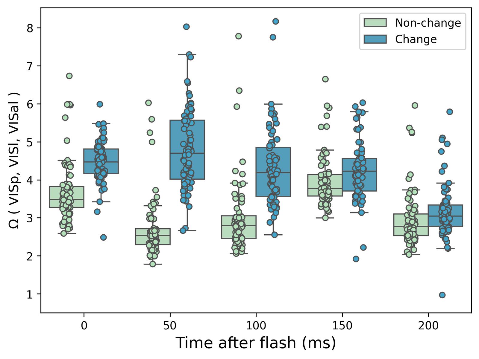
O-information is positive in both conditions, so redundancy dominates. It is higher after an image change than after a repeated image, mostly in the first 100 ms: a new scene is broadcast across the visual areas with more shared information than a repeated one. The same holds with six areas and with 1 ms or 5 ms steps. It is consistent with a partial information decomposition of the same data by Venkatesh et al. (2023), obtained here without choosing sources and a target.
The estimate above pools sessions to have enough training data. ALICE later computed the same quantity separately for every session, with no training on neural data.
References
- M. Bounoua, G. Franzese, P. Michiardi. SΩI: Score-based O-INFORMATION Estimation. ICML 2024 (oral). arXiv:2402.05667, code.
- F. E. Rosas, P. A. M. Mediano, M. Gastpar, H. J. Jensen. Quantifying high-order interdependencies via multivariate extensions of the mutual information. Physical Review E, 2019.
- T. Scagliarini et al. Gradients of O-information: Low-order descriptors of high-order dependencies. Physical Review Research, 2023.
- P. Venkatesh et al. Gaussian partial information decomposition: Bias correction and application to high-dimensional data. NeurIPS 2023.