Estimating mutual information without training
ALICE is a transformer trained once, on synthetic distributions only, that estimates the mutual information of a new dataset directly from its samples, with no training. On the standard benchmark it is more accurate than estimators trained on each task, especially with few samples.
All the estimators in the rest of this series, starting with MINDE, train a model on the data they are asked about. That is fine for one large dataset. It becomes a problem in a study like the visual cortex one below, which needs a separate estimate for every recording session, flash type, and time window: 675 estimates, each from a small sample. With a trained estimator that means 675 training runs, each with its own tuning, on too little data. ALICE gives all 675 from one frozen model, with a few forward passes each.
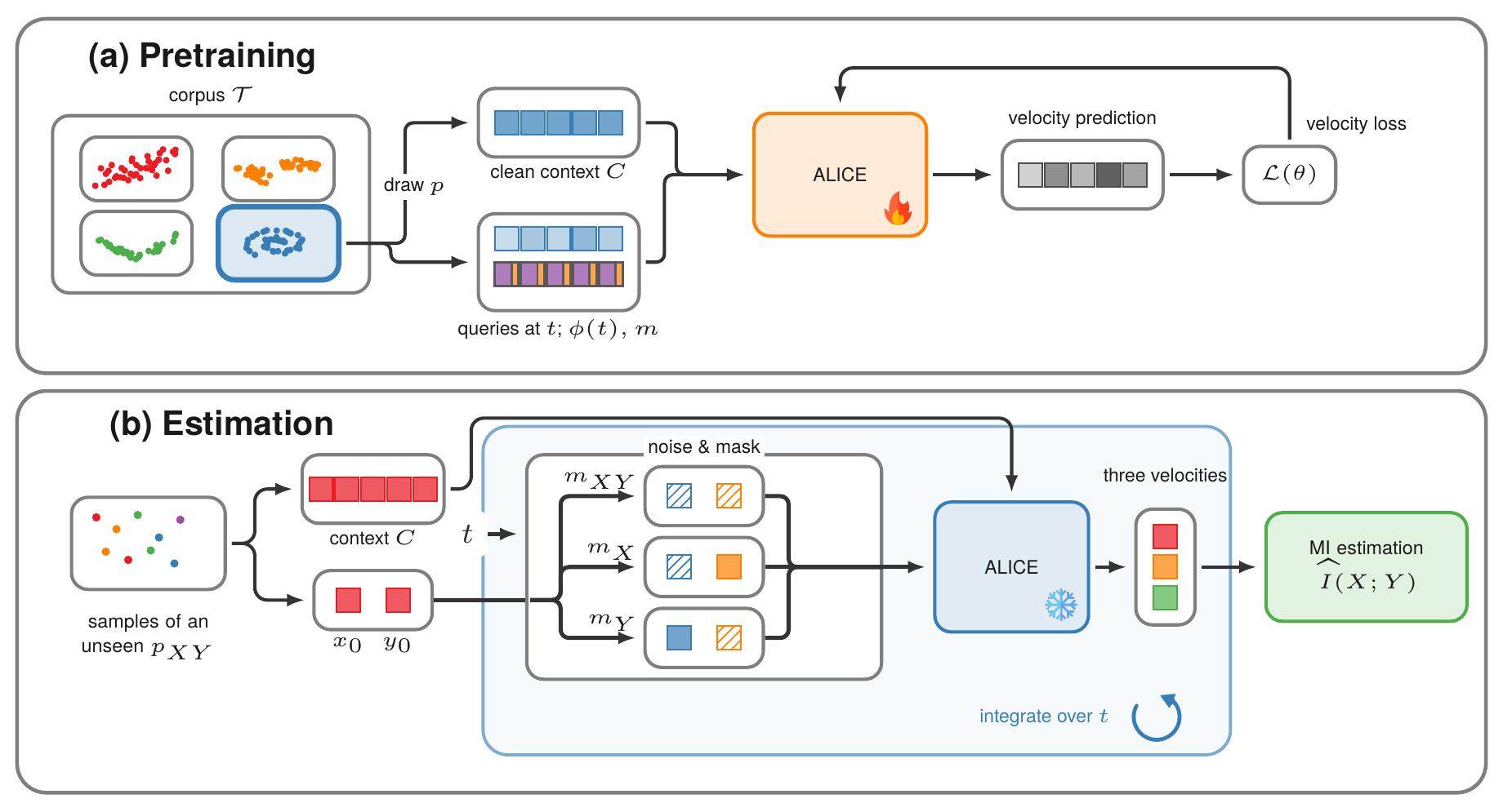
The idea is to learn the estimator itself. ALICE is trained once, on a large collection of synthetic distributions. When it receives samples from a distribution it has never seen, those samples (the context) determine which distribution its output describes, and no parameter is updated.
The identity in velocity form
ALICE uses the rectified-flow version of the identity behind this series. With the interpolant z_t = (1-t)\,z_0 + t\,\epsilon and \epsilon \sim \mathcal N(0, I), the velocity field of a density p is v_t(z) = \mathbb E[z_0 - \epsilon \mid z_t = z], and
\operatorname{KL}(p\,\|\,q) = \int_0^1 \frac{1-t}{t}\; \mathbb E_{z\sim p_t}\big\lVert v^p_t(z) - v^q_t(z) \big\rVert^2\, \mathrm dt .
Velocity and score are related by \nabla \log p_t(z) = \big((1-t)\,v_t(z) - z\big)/t. We work with velocities because the integrand stays bounded at every t, while the score version diverges. For mutual information we compare the joint field with two block-conditional fields, each obtained by noising one block and keeping the other clean:
I(X;Y) = \int_0^1 \frac{1-t}{t}\; \mathbb E\Big[\big\lVert v_t(z_t)|_X - v_t(x_t \mid y_0) \big\rVert^2 + \big\lVert v_t(z_t)|_Y - v_t(y_t \mid x_0) \big\rVert^2 \Big]\,\mathrm dt .
One detail is essential: the three fields must be evaluated with the same noise draw. The proof writes each field as an orthogonal projection of the next, and the projections are orthogonal only when the noise is shared. With independent draws the integrand no longer averages to the mutual information.
From identity to estimator
A single network v_\theta(z, t, m; C) represents all three fields. C is the context of clean samples, and the mask m says which coordinates are noised. For each Monte Carlo draw of a clean pair (x_0, y_0), a time t, and a noise \epsilon,
\hat v = v_\theta(z_t, t, m_{XY}), \quad \hat v_X = v_\theta\big((x_t, y_0), t, m_X\big), \quad \hat v_Y = v_\theta\big((x_0, y_t), t, m_Y\big),
and the estimate is
\hat I(X;Y) = \frac{1}{N_{\mathrm{MC}}} \sum_{i} \frac{1-t_i}{t_i} \Big[ \big\lVert (\hat v - \hat v_X)|_X \big\rVert^2 + \big\lVert (\hat v - \hat v_Y)|_Y \big\rVert^2 \Big].
Before all this, each coordinate is mapped to a standard normal through its empirical CDF on the context. Mutual information does not change under monotone transformations of each coordinate, so this Gaussian-copula step costs nothing, and it puts every dataset on the scale the model was trained on.
Architecture
The same weights have to handle any number of samples n and any number of coordinates d. Four design choices make that possible.
Every scalar coordinate of every sample is a separate token, with an input projection and an output head shared across coordinates, so changing d only changes the number of tokens. There are no positional encodings: the model is invariant to the order of the samples and equivariant to the order of the coordinates, as it should be for a set of exchangeable samples.
Attention over all n context samples would cost \mathcal O(L d n^2). Instead, each coordinate summarizes its context into K = 128 learned latents through cross-attention, which brings the cost down to \mathcal O(d n K + L d K^2), linear in n. The encoded context is computed once and reused by every query.
Which coordinates depend on which changes from one distribution to the next. The model therefore builds a weighted graph over coordinates from covariances of learned nonlinear features of the context, and uses its signed, gated edges to exchange information between coordinates in every layer.
Finally, the parameterization enforces v_0(z) = z exactly. Since the weight (1-t)/t diverges at t = 0, any error there would turn into a systematic positive bias.
Training data
The corpus contains only synthetic distributions, generated from random seeds: copula mixtures of Gaussian and Student-t components, warped Gaussian mixtures, nonparametric regressions with random Fourier features, and noisy manifolds. They cover joint widths from 2 to 100, with 70,000 distributions per width. The loss is masked flow matching, which needs samples and no mutual information labels. ALICE Small (19M parameters) trains in about three days and ALICE Base (85M) in about five and a half, each on two H200 GPUs.
How well it works
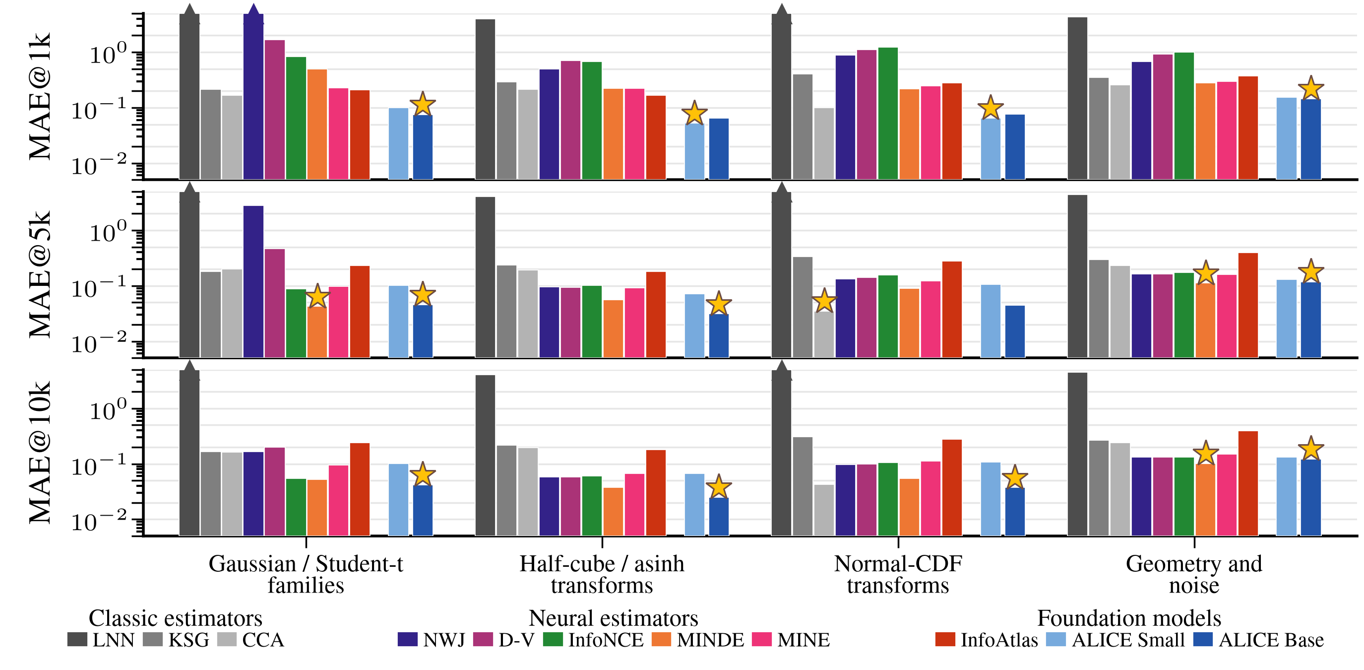
We evaluate on the 40 tasks of the Beyond Normal benchmark (Czyż et al., 2023). Every method gets the same number of samples per task. The trained estimators are trained and tuned on them; ALICE only conditions on them.
| Estimator | 1k | 5k | 10k |
|---|---|---|---|
| ALICE Base | 0.092 | 0.063 | 0.060 |
| ALICE Small | 0.101 | 0.103 | 0.104 |
| InfoAtlas (amortized) | 0.253 | 0.271 | 0.276 |
| MINDE-C (trained per task) | 0.353 | 0.070 | 0.065 |
| MINE (trained per task) | 0.248 | 0.117 | 0.108 |
| CCA (linear) | 0.195 | 0.192 | 0.181 |
ALICE Base has the lowest error at every sample size, and the difference is largest with 1k samples, where it is at least twice as accurate as any other method. With 10k samples, 35 of the 40 tasks are within 0.1 nats of the true value, and the mean signed error is -0.005 nats. The model was trained with contexts of at most 2,048 samples, so the results at 5k and 10k are an extrapolation in context length.
The cost is a handful of forward passes. With 8,192 samples, ALICE Base reaches 0.060 nats for 1.6 \times 10^{13} FLOPs per task; InfoAtlas, the closest amortized estimator, reaches 0.274 nats for 1.9 \times 10^{13}.
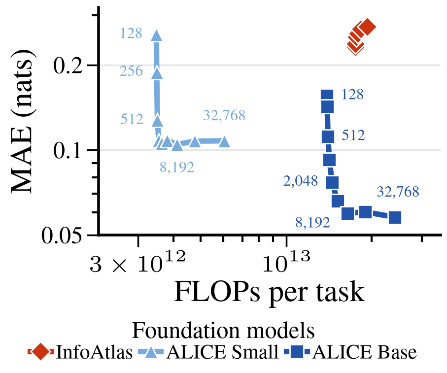
InfoAtlas differs in how it amortizes. It trains a hypernetwork that outputs the weights of a separate variational estimator for each distribution, its input shape is fixed, and it estimates a lower bound. ALICE has no distribution-specific parameters, accepts any number of coordinates, and estimates an exact identity.
Two kinds of tasks account for most of the remaining error. Spiral embeddings are underestimated, by 0.43 and 0.44 nats at joint widths 6 and 10. Dense multinormal tasks are overestimated, by 0.15 nats at width 50 and 0.23 at width 100, and the error grows with the width. ALICE Small makes the same mistakes, by larger amounts. Training on higher-dimensional data and with longer contexts may help with both.
Three applications
None of the following data types appears in the training corpus.
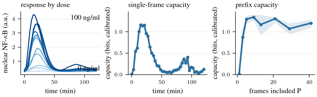
Single-cell signaling. How reliably can a cell tell how much of a stimulus it received? Jetka et al. (2019) imaged 15,632 cells stimulated with one of 11 doses of TNF-α for two hours. From contexts of 1,024 cells, ALICE estimates the channel capacity of the NF-κB pathway. A single frame carries up to about 1.2 bits, at minutes 15 to 21, and the first frames together reach about 1.3 bits by frame 12.
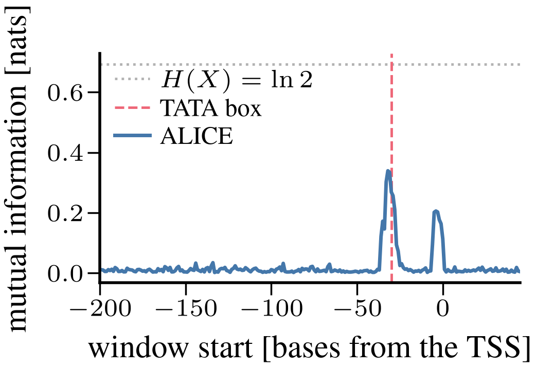
Promoter DNA. The same question as in the INFO-SEDD note, answered without training: the mutual information between a sliding 6-base window and the promoter label of 2,994 Arabidopsis thaliana sequences. The profile is flat except at 30 to 32 bases upstream of the transcription start site, inside the known TATA-box region, with a second peak at the initiator element on the start site.
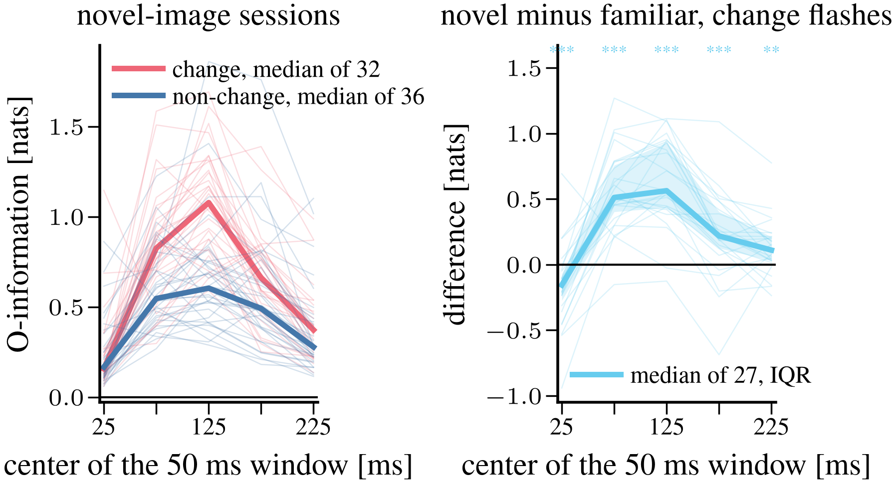
Mouse visual cortex. O-information among six visual areas in the Allen Institute Neuropixels recordings, estimated for each session separately from a context of 128 flashes. Redundancy peaks 100 to 150 ms after a flash, and a novel image raises it: comparing the two sessions of each mouse, the increase appears in 25 of 27 animals for change flashes. Our earlier analysis with SΩI had pooled all sessions into one trained model, which mixes the familiar and novel days of every mouse and cannot separate them.
Using it
from alice import load_model, estimate_mi_fast

model = load_model("eurecom-probai/alice-1.0-base", device="cuda")

# samples: an (N, dx + dy) torch tensor; the two slices select X and Y
mi, std = estimate_mi_fast(
    model, samples, slice(0, dx), slice(dx, dx + dy),
    n_context=N - 64, n_eval=64, return_std=True,
)
print(f"I(X;Y) = {mi:.3f} +/- {std:.3f} nats")
There is also a demo in the browser, and the repository has a tutorial notebook.
References
- G. Franzese, S. Rossi, P. Michiardi. ALICE: In-context, Zero-shot, Mutual Information Estimation. Preprint, 2026. arXiv:2609.34962, code.
- P. Czyż, F. Grabowski, J. E. Vogt, N. Beerenwinkel, A. Marx. Beyond Normal: On the Evaluation of Mutual Information Estimators. NeurIPS 2023.
- T. Jetka et al. Information-theoretic analysis of multivariate single-cell signaling responses. PLoS Computational Biology, 2019.