Estimating mutual information
MINDE (ICLR 2024) estimates mutual information as an integrated squared difference between the scores of a diffusion model, with a single network providing all of them. Trained on 100k samples, it is within 0.1 nats of the true value on 35 of the 40 tasks of the standard benchmark, and it passes the self-consistency tests that many neural estimators fail.
Suppose you observe pairs (x_i, y_i) and want to decide whether they come from the joint distribution p_{XY} or from the product of the marginals p_X \otimes p_Y, that is, from independent X and Y. The best test you can build has an error that decays exponentially with the number of pairs (Stein’s lemma), and the exponent is the mutual information
I(X;Y) = \operatorname{KL}\big(p_{XY} \,\|\, p_X \otimes p_Y\big).
Equivalently, mutual information is the rate at which dependence becomes detectable. It is zero only under independence, it is unchanged by smooth invertible transformations of X or of Y, and it sees nonlinear dependence that a correlation coefficient misses. In biology and neuroscience the question is often exactly this one, how many bits a response carries about a stimulus.
Why it is hard
There are two easy cases. For jointly Gaussian variables with covariance blocks \Sigma_{XX} and \Sigma_{YY} and joint covariance \Sigma,
I(X;Y) = \tfrac12 \log \frac{\det \Sigma_{XX}\,\det \Sigma_{YY}}{\det \Sigma},
and for discrete variables with few values one can count. Beyond that, the classical estimators degrade quickly. Binning needs a sample that grows exponentially with the dimension. The Kraskov-Stögbauer-Grassberger nearest-neighbor estimator is good in a few dimensions and biased in many. A Gaussian fit only captures the linear part of the dependence.
Neural estimators learn the density ratio instead, and each family has its own limit. MINE, NWJ, and Donsker-Varadhan train a critic T to maximize \mathbb E_{p_{XY}}[T] - \log \mathbb E_{p_X\otimes p_Y}[e^T]; the second term averages an exponential, is dominated by rare samples, and makes the estimate noisy or divergent. InfoNCE is stable but cannot exceed \log N for a batch of N samples. More generally, McAllester and Stratos (2020) showed that a high-confidence lower bound above \log N nats cannot be certified from N samples, so bounds are a poor tool when the mutual information is large.
MINDE
The identity behind this series writes a KL divergence as an integrated squared difference of two scores. Applied to mutual information it gives two estimators, depending on which pair of distributions we compare.
The conditional version, MINDE-C, uses I(X;Y) = \mathbb E_{Y}\big[\operatorname{KL}(p_{X\mid Y} \,\|\, p_X)\big] and diffuses only X:
I(X;Y) = \int_0^T \mathbb E\Big[\big\lVert \nabla \log p_t(X_t \mid Y) - \nabla \log p_t(X_t) \big\rVert^2\Big]\,\mathrm dt.
The joint version, MINDE-J, diffuses X and Y together and compares the joint score with the two marginal scores stacked side by side:
I(X;Y) = \int_0^T \mathbb E\Big[\big\lVert \nabla \log p_t(X_t, Y_t) - \big(\nabla \log p_t(X_t),\, \nabla \log p_t(Y_t)\big) \big\rVert^2\Big]\,\mathrm dt.
We train one network for all the scores. A flag c tells it whether to return the conditional score (c=1, with Y as input) or the marginal one (c=0, with Y masked), so training is ordinary denoising with random masking. For MINDE-C, estimation then fits in a few lines:
(a, b)  ~ p_XY                                 # a data pair
t       ~ Uniform[0, T]
x_t     = exp(-t) a + sqrt(1 - exp(-2t)) eps,  eps ~ N(0, I)
s_marg  = net([x_t, 0], t, c=0)                # score of p_t(x)
s_cond  = net([x_t, b], t, c=1)                # score of p_t(x | b)
I_hat   = T * || s_marg - s_cond ||^2          # averaged over many draws
The same network also gives the entropies h(X) and h(X\mid Y), since each is a KL divergence to a Gaussian reference plus a constant.
The benchmark with ground truth
The Beyond Normal benchmark (Czyż et al., 2023) has 40 tasks with known mutual information: 10 distributions in 4 parametrizations, including sparse multinormals, heavy-tailed Student-t distributions, and transformations such as half-cube, normal CDF, Swiss roll, and spiral embeddings that leave mutual information unchanged but distort the data. The original benchmark trains each method on 10k samples, which is often not enough for the neural baselines to give stable estimates. In the MINDE paper we therefore train every method on 100k samples, with comparable numbers of parameters, and average over 10 seeds.
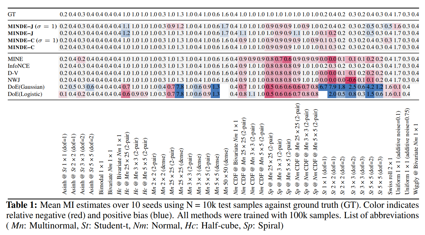
With this budget, MINDE-C is within 0.1 nats of the true value on 35 of the 40 tasks. MINE, the next best, reaches 24 of 40. The baselines are least accurate on heavy-tailed distributions (Student-t) and strong transformations (spiral, normal CDF), where MINDE remains accurate. On a separate benchmark with high mutual information, built from sparse multinormals, all neural estimators follow the ground truth on the untransformed data, and MINDE is the most accurate once half-cube or spiral transformations are applied.
Self-consistency on images
A benchmark with ground truth has to use synthetic distributions, which leaves open how an estimator behaves on real high-dimensional data. Self-consistency tests address this without needing the true value. Following Song and Ermon (2020), we take MNIST images and let Y be the top t rows of the image X.
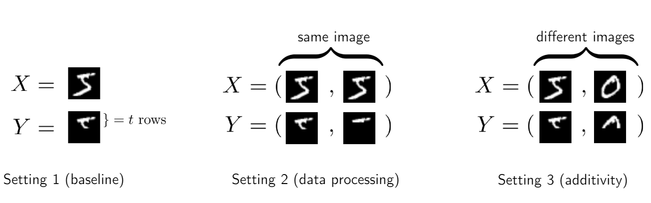
Each test has a known answer for a ratio of estimates:
- Baseline. Revealing more rows can only add information, so the estimate should grow with t and approach its value for the full image (ratio 1).
- Data processing. A processed copy of Y carries no new information about X, so adding it should leave the estimate unchanged (ratio 1).
- Additivity. Two independent pairs carry twice the information of one (ratio 2).
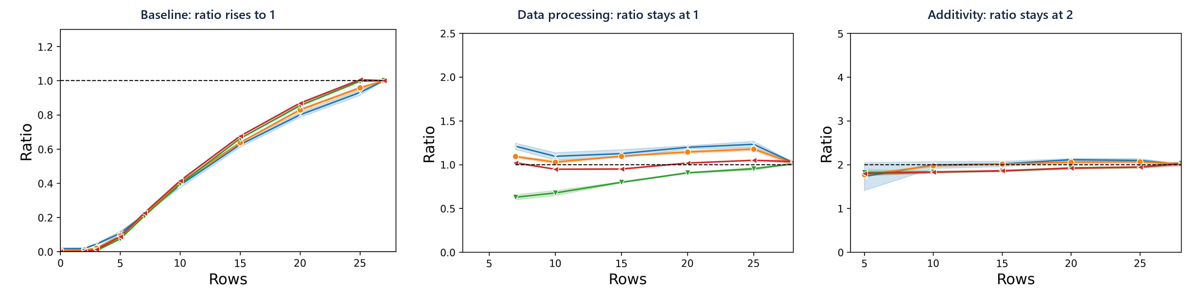
MINDE passes all three, which several variational estimators do not.
How many samples does it need?
The benchmark above uses 100k samples, a large budget. Every estimator, MINDE included, trains a model on the data at hand, so with fewer samples all of them lose accuracy. The mean absolute error on the same 40 tasks, with smaller budgets that are the same for every method:
| Estimator | 1k samples | 5k samples | 10k samples |
|---|---|---|---|
| MINDE-C | 0.353 | 0.070 | 0.065 |
| MINE | 0.248 | 0.117 | 0.108 |
| InfoNCE | 0.887 | 0.123 | 0.083 |
| KSG | 0.288 | 0.240 | 0.219 |
| CCA (linear) | 0.195 | 0.192 | 0.181 |
From 5k samples on, MINDE is the most accurate of this group. At 1k samples every trained estimator loses accuracy, and the linear baseline is the best of the group. Many biological datasets have about a thousand samples per condition or fewer. This small-sample regime motivated ALICE, a model trained once that estimates mutual information directly from the samples, and reaches 0.092 nats at 1k samples on the same benchmark.
Text-to-image alignment
Mutual information also has uses outside science. The mutual information between a text description and a generated image measures how much of the description the image reflects. In Information Theoretic Text-to-Image Alignment (ICLR 2025) we estimate its pointwise version with the denoising network of the text-to-image model itself, and use it to select the generations that best match their text descriptions as a fine-tuning set. No human annotation and no external vision-language model are involved. RFMI extends the same estimator to rectified-flow models.
Choosing an estimator
For a quick look at low-dimensional data with plenty of samples, KSG is a reasonable first try. With a few thousand samples or more, or when the quantity of interest goes beyond mutual information, MINDE and its relatives (SΩI, TENDE, INFO-SEDD) are the better choice. With few samples, many datasets, or no wish to train anything, use ALICE.
References
- G. Franzese, M. Bounoua, P. Michiardi. MINDE: Mutual Information Neural Diffusion Estimation. ICLR 2024. arXiv:2310.09031, code.
- C. Wang, G. Franzese, A. Finamore, M. Gallo, P. Michiardi. Information Theoretic Text-to-Image Alignment. ICLR 2025. arXiv:2405.20759.
- P. Czyż, F. Grabowski, J. E. Vogt, N. Beerenwinkel, A. Marx. Beyond Normal: On the Evaluation of Mutual Information Estimators. NeurIPS 2023.
- D. McAllester, K. Stratos. Formal Limitations on the Measurement of Mutual Information. AISTATS 2020.
- J. Song, S. Ermon. Understanding the Limitations of Variational Mutual Information Estimators. ICLR 2020.